
Data Analysis: Game of Thrones (Fun)
Game of Thrones
I happened to bump into a Game of Thrones data set and decided it would interesting to see what was going on there. I recently watched the seasons 1 - 7, under duress at first. But slowly realised the genius and brilliance of George RR Martin.
import numpy as np # linear algebra
import pandas as pd # data processing, CSV file I/O (e.g. pd.read_csv)
import seaborn as sn # data visualization
import matplotlib.pyplot as ml # data visualisation as well
import warnings


sn.set(color_codes = True, style="white")
battles = pd.read_csv("battles.csv", sep=",", header=0)
deaths = pd.read_csv("character-deaths.csv", sep=",", header=0)
predictions = pd.read_csv("character-predictions.csv", sep=",", header=0)
We look at the basic shape of the data sets
battles.shape
(38, 25)
deaths.shape
(917, 13)
predictions.shape
(1946, 33)
Lets have a peek at what we are working with.
battles.head()
| name | year | battle_number | attacker_king | defender_king | attacker_1 | attacker_2 | attacker_3 | attacker_4 | defender_1 | ... | major_death | major_capture | attacker_size | defender_size | attacker_commander | defender_commander | summer | location | region | note | |
|---|---|---|---|---|---|---|---|---|---|---|---|---|---|---|---|---|---|---|---|---|---|
| 0 | Battle of the Golden Tooth | 298 | 1 | Joffrey/Tommen Baratheon | Robb Stark | Lannister | NaN | NaN | NaN | Tully | ... | 1.0 | 0.0 | 15000.0 | 4000.0 | Jaime Lannister | Clement Piper, Vance | 1.0 | Golden Tooth | The Westerlands | NaN |
| 1 | Battle at the Mummer's Ford | 298 | 2 | Joffrey/Tommen Baratheon | Robb Stark | Lannister | NaN | NaN | NaN | Baratheon | ... | 1.0 | 0.0 | NaN | 120.0 | Gregor Clegane | Beric Dondarrion | 1.0 | Mummer's Ford | The Riverlands | NaN |
| 2 | Battle of Riverrun | 298 | 3 | Joffrey/Tommen Baratheon | Robb Stark | Lannister | NaN | NaN | NaN | Tully | ... | 0.0 | 1.0 | 15000.0 | 10000.0 | Jaime Lannister, Andros Brax | Edmure Tully, Tytos Blackwood | 1.0 | Riverrun | The Riverlands | NaN |
| 3 | Battle of the Green Fork | 298 | 4 | Robb Stark | Joffrey/Tommen Baratheon | Stark | NaN | NaN | NaN | Lannister | ... | 1.0 | 1.0 | 18000.0 | 20000.0 | Roose Bolton, Wylis Manderly, Medger Cerwyn, H... | Tywin Lannister, Gregor Clegane, Kevan Lannist... | 1.0 | Green Fork | The Riverlands | NaN |
| 4 | Battle of the Whispering Wood | 298 | 5 | Robb Stark | Joffrey/Tommen Baratheon | Stark | Tully | NaN | NaN | Lannister | ... | 1.0 | 1.0 | 1875.0 | 6000.0 | Robb Stark, Brynden Tully | Jaime Lannister | 1.0 | Whispering Wood | The Riverlands | NaN |
5 rows × 23 columns
deaths.head()
Index(['Name', 'Allegiances', 'Death Year', 'Book of Death', 'Death Chapter',
       'Book Intro Chapter', 'Gender', 'Nobility', 'GoT', 'CoK', 'SoS', 'FfC',
       'DwD'],
      dtype='object')
predictions.head()
Index(['S.No', 'actual', 'pred', 'alive', 'plod', 'name', 'title', 'male',
       'culture', 'dateOfBirth', 'DateoFdeath', 'mother', 'father', 'heir',
       'house', 'spouse', 'book1', 'book2', 'book3', 'book4', 'book5',
       'isAliveMother', 'isAliveFather', 'isAliveHeir', 'isAliveSpouse',
       'isMarried', 'isNoble', 'age', 'numDeadRelations', 'boolDeadRelations',
       'isPopular', 'popularity', 'isAlive'],
      dtype='object')
Basic Statistical Analysis of the data sets.
battles.describe()
| year | battle_number | major_death | major_capture | attacker_size | defender_size | summer | |
|---|---|---|---|---|---|---|---|
| count | 38.000000 | 38.000000 | 37.000000 | 37.000000 | 24.000000 | 19.000000 | 37.000000 |
| mean | 299.105263 | 19.500000 | 0.351351 | 0.297297 | 9942.541667 | 6428.157895 | 0.702703 |
| std | 0.689280 | 11.113055 | 0.483978 | 0.463373 | 20283.092065 | 6225.182106 | 0.463373 |
| min | 298.000000 | 1.000000 | 0.000000 | 0.000000 | 20.000000 | 100.000000 | 0.000000 |
| 25% | 299.000000 | 10.250000 | 0.000000 | 0.000000 | 1375.000000 | 1070.000000 | 0.000000 |
| 50% | 299.000000 | 19.500000 | 0.000000 | 0.000000 | 4000.000000 | 6000.000000 | 1.000000 |
| 75% | 300.000000 | 28.750000 | 1.000000 | 1.000000 | 8250.000000 | 10000.000000 | 1.000000 |
| max | 300.000000 | 38.000000 | 1.000000 | 1.000000 | 100000.000000 | 20000.000000 | 1.000000 |
Columns (defender_3, defender_4) are basically empty and irrelevant so we can drop them.
battles = battles.drop(['defender_3', 'defender_4'],1)
deaths.describe()
| Death Year | Book of Death | Death Chapter | Book Intro Chapter | Gender | Nobility | GoT | CoK | SoS | FfC | DwD | |
|---|---|---|---|---|---|---|---|---|---|---|---|
| count | 305.000000 | 307.000000 | 299.000000 | 905.000000 | 917.000000 | 917.000000 | 917.000000 | 917.000000 | 917.000000 | 917.000000 | 917.000000 |
| mean | 299.157377 | 2.928339 | 40.070234 | 28.861878 | 0.828790 | 0.468920 | 0.272628 | 0.353326 | 0.424209 | 0.272628 | 0.284624 |
| std | 0.703483 | 1.326482 | 20.470270 | 20.165788 | 0.376898 | 0.499305 | 0.445554 | 0.478264 | 0.494492 | 0.445554 | 0.451481 |
| min | 297.000000 | 1.000000 | 0.000000 | 0.000000 | 0.000000 | 0.000000 | 0.000000 | 0.000000 | 0.000000 | 0.000000 | 0.000000 |
| 25% | 299.000000 | 2.000000 | 25.500000 | 11.000000 | 1.000000 | 0.000000 | 0.000000 | 0.000000 | 0.000000 | 0.000000 | 0.000000 |
| 50% | 299.000000 | 3.000000 | 39.000000 | 27.000000 | 1.000000 | 0.000000 | 0.000000 | 0.000000 | 0.000000 | 0.000000 | 0.000000 |
| 75% | 300.000000 | 4.000000 | 57.000000 | 43.000000 | 1.000000 | 1.000000 | 1.000000 | 1.000000 | 1.000000 | 1.000000 | 1.000000 |
| max | 300.000000 | 5.000000 | 80.000000 | 80.000000 | 1.000000 | 1.000000 | 1.000000 | 1.000000 | 1.000000 | 1.000000 | 1.000000 |
predictions.describe()
| S.No | actual | pred | alive | plod | male | dateOfBirth | DateoFdeath | book1 | book2 | ... | isAliveHeir | isAliveSpouse | isMarried | isNoble | age | numDeadRelations | boolDeadRelations | isPopular | popularity | isAlive | |
|---|---|---|---|---|---|---|---|---|---|---|---|---|---|---|---|---|---|---|---|---|---|
| count | 1946.000000 | 1946.000000 | 1946.000000 | 1946.000000 | 1946.000000 | 1946.000000 | 433.000000 | 444.000000 | 1946.000000 | 1946.000000 | ... | 23.000000 | 276.000000 | 1946.000000 | 1946.000000 | 433.000000 | 1946.000000 | 1946.000000 | 1946.000000 | 1946.000000 | 1946.000000 |
| mean | 973.500000 | 0.745632 | 0.687050 | 0.634470 | 0.365530 | 0.619219 | 1577.364896 | 2950.193694 | 0.198356 | 0.374615 | ... | 0.652174 | 0.778986 | 0.141829 | 0.460946 | -1293.563510 | 0.305755 | 0.074512 | 0.059096 | 0.089584 | 0.745632 |
| std | 561.906131 | 0.435617 | 0.463813 | 0.312637 | 0.312637 | 0.485704 | 19565.414460 | 28192.245529 | 0.398864 | 0.484148 | ... | 0.486985 | 0.415684 | 0.348965 | 0.498601 | 19564.340993 | 1.383910 | 0.262669 | 0.235864 | 0.160568 | 0.435617 |
| min | 1.000000 | 0.000000 | 0.000000 | 0.000000 | 0.000000 | 0.000000 | -28.000000 | 0.000000 | 0.000000 | 0.000000 | ... | 0.000000 | 0.000000 | 0.000000 | 0.000000 | -298001.000000 | 0.000000 | 0.000000 | 0.000000 | 0.000000 | 0.000000 |
| 25% | 487.250000 | 0.000000 | 0.000000 | 0.391250 | 0.101000 | 0.000000 | 240.000000 | 282.000000 | 0.000000 | 0.000000 | ... | 0.000000 | 1.000000 | 0.000000 | 0.000000 | 18.000000 | 0.000000 | 0.000000 | 0.000000 | 0.013378 | 0.000000 |
| 50% | 973.500000 | 1.000000 | 1.000000 | 0.735500 | 0.264500 | 1.000000 | 268.000000 | 299.000000 | 0.000000 | 0.000000 | ... | 1.000000 | 1.000000 | 0.000000 | 0.000000 | 27.000000 | 0.000000 | 0.000000 | 0.000000 | 0.033445 | 1.000000 |
| 75% | 1459.750000 | 1.000000 | 1.000000 | 0.899000 | 0.608750 | 1.000000 | 285.000000 | 299.000000 | 0.000000 | 1.000000 | ... | 1.000000 | 1.000000 | 0.000000 | 1.000000 | 50.000000 | 0.000000 | 0.000000 | 0.000000 | 0.086957 | 1.000000 |
| max | 1946.000000 | 1.000000 | 1.000000 | 1.000000 | 1.000000 | 1.000000 | 298299.000000 | 298299.000000 | 1.000000 | 1.000000 | ... | 1.000000 | 1.000000 | 1.000000 | 1.000000 | 100.000000 | 15.000000 | 1.000000 | 1.000000 | 1.000000 | 1.000000 |
8 rows × 25 columns
We will now see if we have any relationships between variables
battles.corr()
| year | battle_number | major_death | major_capture | attacker_size | defender_size | summer | |
|---|---|---|---|---|---|---|---|
| year | 1.000000 | 0.906781 | -0.341050 | -0.166234 | 0.155841 | -0.366048 | -0.841912 |
| battle_number | 0.906781 | 1.000000 | -0.270421 | -0.105225 | 0.086418 | -0.297730 | -0.799090 |
| major_death | -0.341050 | -0.270421 | 1.000000 | 0.264464 | 0.267966 | 0.081815 | 0.337136 |
| major_capture | -0.166234 | -0.105225 | 0.264464 | 1.000000 | 0.331961 | 0.249510 | 0.142112 |
| attacker_size | 0.155841 | 0.086418 | 0.267966 | 0.331961 | 1.000000 | -0.112118 | -0.273054 |
| defender_size | -0.366048 | -0.297730 | 0.081815 | 0.249510 | -0.112118 | 1.000000 | 0.347108 |
| summer | -0.841912 | -0.799090 | 0.337136 | 0.142112 | -0.273054 | 0.347108 | 1.000000 |
ml.figure(figsize=(20,10))
sn.heatmap(battles.corr(),annot=True)
<matplotlib.axes._subplots.AxesSubplot at 0xba67550>
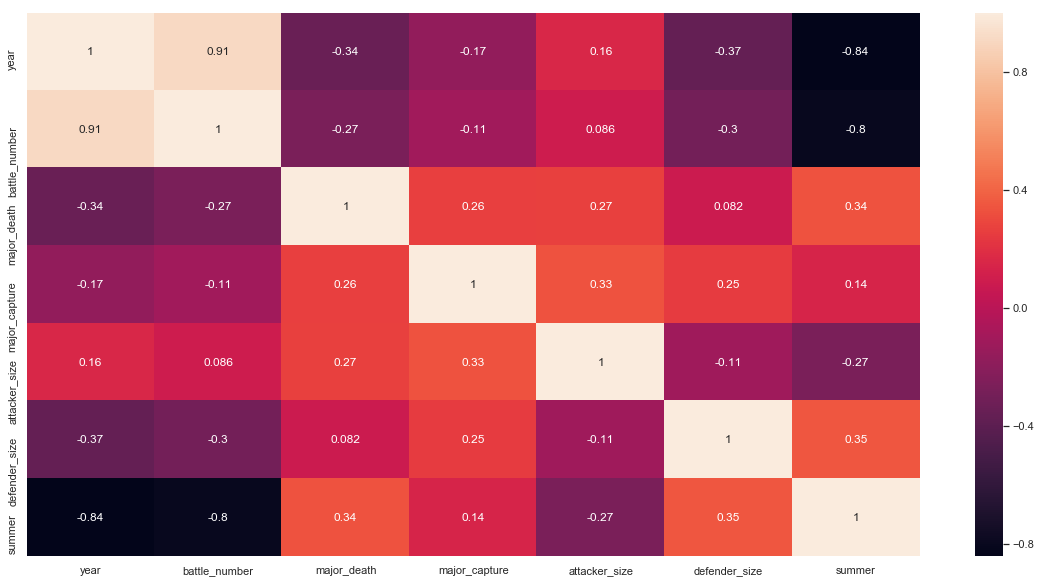
There seems to be no correlation between any variables
deaths.corr()
| Death Year | Book of Death | Death Chapter | Book Intro Chapter | Gender | Nobility | GoT | CoK | SoS | FfC | DwD | |
|---|---|---|---|---|---|---|---|---|---|---|---|
| Death Year | 1.000000 | 0.832274 | -0.068763 | 0.051674 | -0.135058 | 0.042457 | -0.439234 | 0.077509 | 0.313062 | 0.357204 | 0.550213 |
| Book of Death | 0.832274 | 1.000000 | -0.207666 | 0.016975 | -0.111461 | 0.017475 | -0.434004 | -0.131860 | 0.350095 | 0.340436 | 0.714574 |
| Death Chapter | -0.068763 | -0.207666 | 1.000000 | 0.388283 | -0.086533 | 0.075943 | 0.126657 | 0.012939 | -0.149095 | -0.167285 | -0.145384 |
| Book Intro Chapter | 0.051674 | 0.016975 | 0.388283 | 1.000000 | 0.058684 | -0.068825 | 0.129241 | 0.002445 | 0.158419 | -0.146165 | -0.077509 |
| Gender | -0.135058 | -0.111461 | -0.086533 | 0.058684 | 1.000000 | -0.060213 | 0.070228 | 0.063424 | -0.049199 | -0.040289 | -0.046924 |
| Nobility | 0.042457 | 0.017475 | 0.075943 | -0.068825 | -0.060213 | 1.000000 | 0.087201 | 0.055179 | 0.046825 | 0.146088 | -0.001880 |
| GoT | -0.439234 | -0.434004 | 0.126657 | 0.129241 | 0.070228 | 0.087201 | 1.000000 | 0.121257 | 0.004696 | -0.088852 | -0.120242 |
| CoK | 0.077509 | -0.131860 | 0.012939 | 0.002445 | 0.063424 | 0.055179 | 0.121257 | 1.000000 | -0.002049 | -0.083669 | -0.107276 |
| SoS | 0.313062 | 0.350095 | -0.149095 | 0.158419 | -0.049199 | 0.046825 | 0.004696 | -0.002049 | 1.000000 | -0.074585 | -0.013294 |
| FfC | 0.357204 | 0.340436 | -0.167285 | -0.146165 | -0.040289 | 0.146088 | -0.088852 | -0.083669 | -0.074585 | 1.000000 | -0.109387 |
| DwD | 0.550213 | 0.714574 | -0.145384 | -0.077509 | -0.046924 | -0.001880 | -0.120242 | -0.107276 | -0.013294 | -0.109387 | 1.000000 |
ml.figure(figsize=(20,10))
sn.heatmap(deaths.corr(),annot=True)
<matplotlib.axes._subplots.AxesSubplot at 0xc42de10>
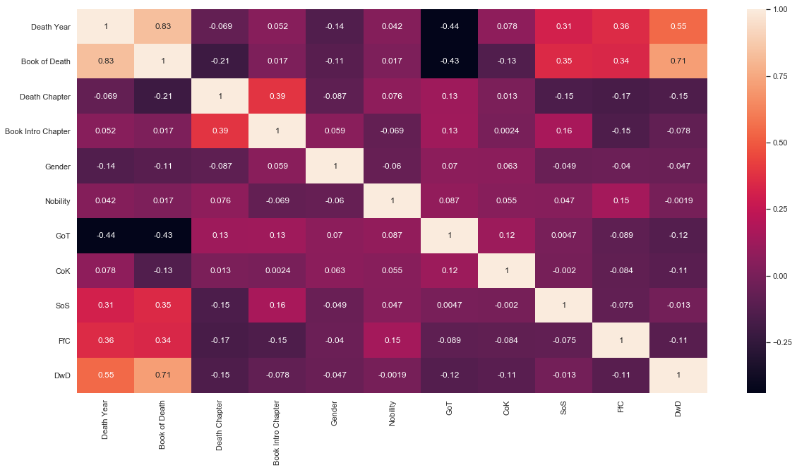
There seems to be a decent correlation between the Death Year and Book (DWD) Dancing with Dragons and Book of Death.
Battles
When we look at the battles lets see who is winning.
ml.figure(figsize = (15,10))
sn.countplot(x='attacker_outcome',data = battles)
<matplotlib.axes._subplots.AxesSubplot at 0xbb6cd30>
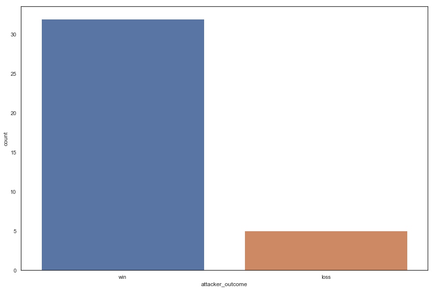
We can say chances are if you start a battle you will likely win. Which makes sense, because one would never start a battle if they did not feel more than prepared. Also you would never attack your opponent when they expect it.
ml.figure(figsize = (15,10))
attack = pd.DataFrame(battles.groupby("attacker_king").size().sort_values())
attack = attack.rename(columns = {0:'Battle'})
attack.plot(kind='bar')
<matplotlib.axes._subplots.AxesSubplot at 0xbda3dd8>


<Figure size 1080x720 with 0 Axes>
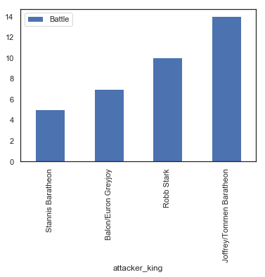
If you have watched the series you will not be surprised by this. I am still surprised that Robb Stark had that many battles that he started
ml.figure(figsize = (15,10))
attack = pd.DataFrame(battles.groupby("defender_king").size().sort_values())
attack = attack.rename(columns = {0:'Defenece'})
attack.plot(kind='bar')
<matplotlib.axes._subplots.AxesSubplot at 0xc75b550>


<Figure size 1080x720 with 0 Axes>
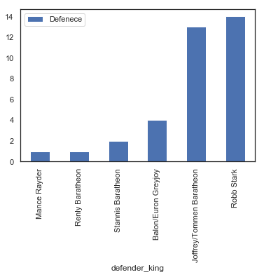
The Baratheon’s seemed to be able to give as good as they get. Again Surprised Robb had to defend himself so many times considering he was so close to the North.
We will now look at the various win loss ratios.
ml.figure(figsize = (15,10))
sn.countplot(x='attacker_king', hue = 'attacker_outcome', data = battles)
<matplotlib.axes._subplots.AxesSubplot at 0xccc4400>
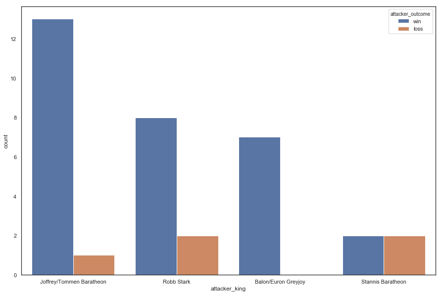
Everyone had decent win ratios bar Stannis Baratheon.
ml.figure(figsize = (15,10))
sn.countplot(x='attacker_outcome', hue= 'battle_type', data = battles)
ml.legend(bbox_to_anchor=(1, 1), loc=2)
<matplotlib.legend.Legend at 0x10dfd780>
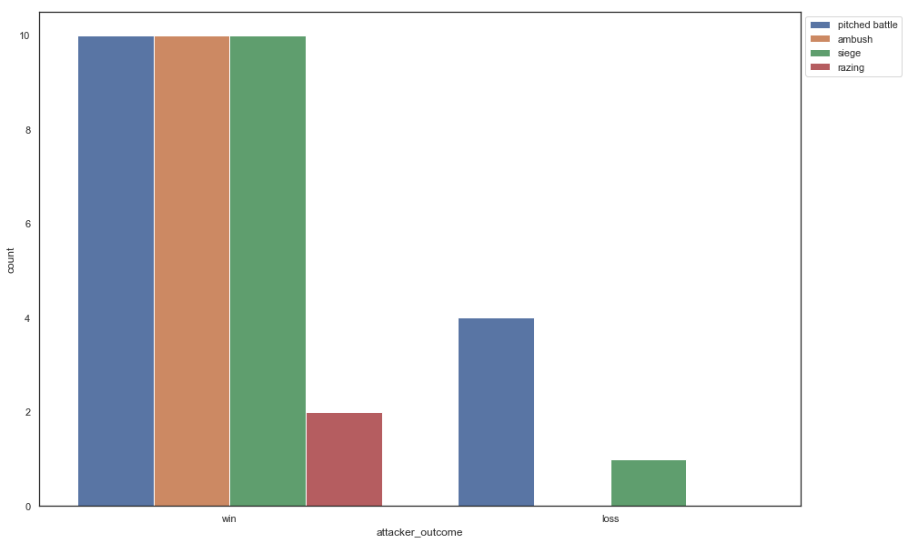
Seems like sieges and razings had a best success ratios, 100%, whereas pitched battles were nearly 50/50.
ml.figure(figsize = (15,10))
sn.countplot(x='year', data = battles)
<matplotlib.axes._subplots.AxesSubplot at 0x10bc2128>
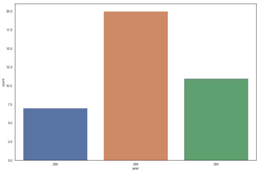
The year 299 had the battles. Why? I do not know.